
Problem Statement
The Human Activity Recognition database was built from the recordings of 30 study participants performing activities of daily living (ADL) while carrying a waist-mounted smartphone with embedded inertial sensors. The objective is to classify activities into one of the six activities performed.
About Dataset
The experiments have been carried out with a group of 30 volunteers within an age bracket of 19-48 years. Each person performed six activities (WALKING, WALKINGUPSTAIRS, WALKINGDOWNSTAIRS, SITTING, STANDING, LAYING) wearing a smartphone (Samsung Galaxy S II) on the waist. Using its embedded accelerometer and gyroscope, we captured 3-axial linear acceleration and 3-axial angular velocity at a constant rate of 50Hz. The experiments have been video-recorded to label the data manually. The obtained dataset has been randomly partitioned into two sets, where 70% of the volunteers was selected for generating the training data and 30% the test data.
The sensor signals (accelerometer and gyroscope) were pre-processed by applying noise filters and then sampled in fixed-width sliding windows of 2.56 sec and 50% overlap (128 readings/window). The sensor acceleration signal, which has gravitational and body motion components, was separated using a Butterworth low-pass filter into body acceleration and gravity. The gravitational force is assumed to have only low frequency components, therefore a filter with 0.3 Hz cutoff frequency was used. From each window, a vector of features was obtained by calculating variables from the time and frequency domain.
Attribute information
For each record in the dataset the following is provided:
-
Triaxial acceleration from the accelerometer (total acceleration) and the estimated body acceleration.
-
Triaxial Angular velocity from the gyroscope.
-
A 561-feature vector with time and frequency domain variables.
-
Its activity label.
-
An identifier of the subject who carried out the experiment.
Importing libraries
import pandas as pd
import numpy as np
import os
import matplotlib.pyplot as plt
import seaborn as sns
from sklearn.model_selection import train_test_split
from sklearn.preprocessing import LabelEncoder
from sklearn.svm import SVC
from sklearn.metrics import precision_recall_fscore_support as error_metric
from sklearn.metrics import confusion_matrix, accuracy_score
from sklearn.feature_selection import SelectFromModel
from sklearn.model_selection import GridSearchCV
from sklearn.svm import LinearSVC
import warnings
warnings.filterwarnings('ignore')
1. EDA
1.1 Loading Dataset ,checking for null values and statistical description
The first step - you know the drill by now - load the dataset and see how it looks like. In this task, we are basically looking for descriptive statistics of overall data and look at the null values if they are present. Since the data is too large I will be only printiing till 25 columns.
data = pd.read_csv('file.csv')
print('Null Values In DataFrame: {}\n'.format(data.isna().sum().sum()))
data.describe().T[:25]
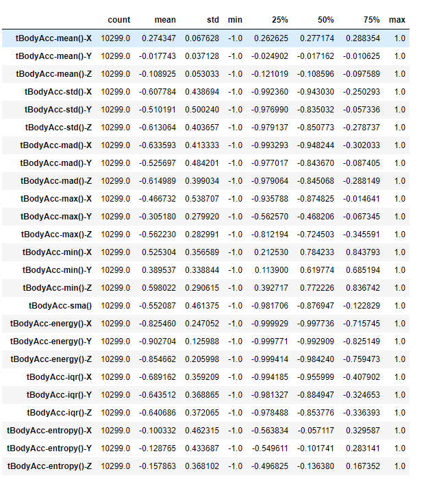
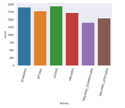
We have 563 features and 10299 rows
Observation:
After observing the dataset statistical description majority of the values are having a minimum value of -1 and maximum value of 1 which brings us to the conclusion that scaling is not required in this case. Also the data set is free of any kind of null values.
-
1.2 Distribution of our class
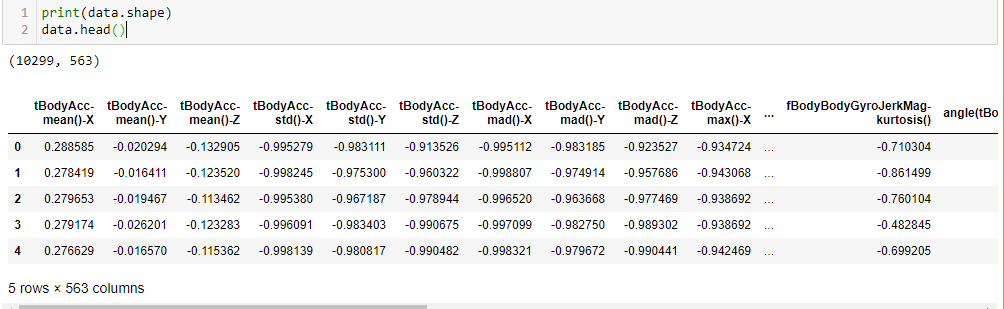
Let’s get a little bit deeper dive into exploring the target feature via graphical methods.
label = data['Activity']
sns.countplot(x= label)
plt.xticks(rotation=75);
Observation:
The class distribution are somewhat balanced which is a better thing on prediction and model building part.
-
1.3 How Long Does The Participant Use The Staircase?
Since the dataset has been created in an scientific environment nearly equal preconditions for the participants can be assumed. It is highly likely for the participants to have been walking up and down the same number of staircases. Bascially we are looking to calculate how much time the each participant has been spending while walking downstairs and upstairs as it seems to be most frequent activity. Let us investigate their activity durations. The description of the data states; “fixed-width sliding windows of 2.56 sec and 50% overlap” for each datapoint.Therefore a single datapoint is gathered every 1.28 sec.
data_copy = data.copy()
data_copy['duration'] = ''
duration_df = (data_copy.groupby([label[label.isin(['WALKING_UPSTAIRS', 'WALKING_DOWNSTAIRS'])], 'subject'])['duration'].count() * 1.28)
duration_df = pd.DataFrame(duration_df)
plot_data = duration_df.reset_index().sort_values('duration', ascending=False)
plot_data['Activity'] = plot_data['Activity'].map({'WALKING_UPSTAIRS':'Upstairs', 'WALKING_DOWNSTAIRS':'Downstairs'})
plt.figure(figsize=(15,5))
sns.barplot(data=plot_data, x='subject', y='duration', hue='Activity')
plt.title('Participants Compared By Their Staircase Walking Duration')
plt.xlabel('Participants')
plt.ylabel('Total Duration [s]')
plt.show()
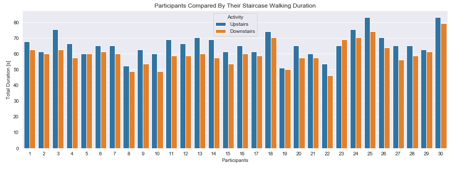
Observation:
Nearly all participants have more data for walking upstairs than downstairs. Assuming an equal number of up- and down-walks the participants need longer walking upstairs. Furthermore the range of the duration is narrow and adjusted to the conditions. A young person being ~50% fast in walking upstairs than an older one is reasonable.
-
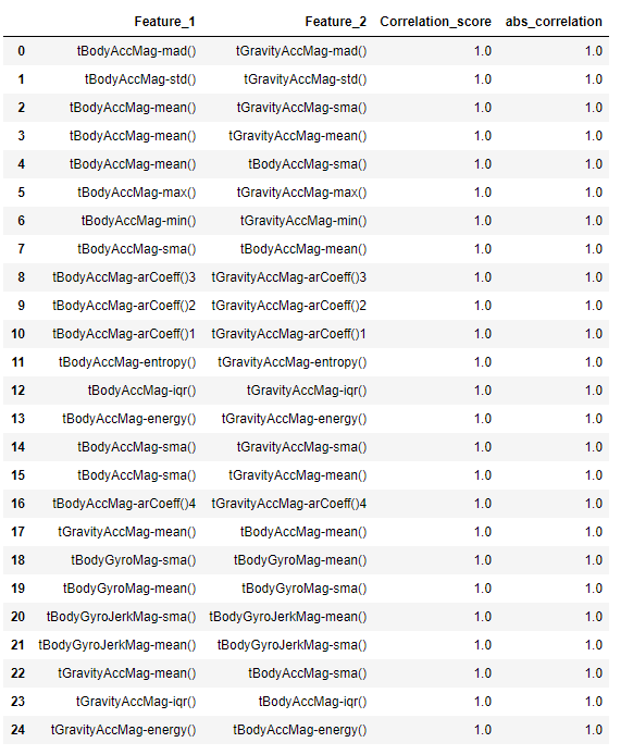
1.4 Finding the correlation
We always try to reduce our features to the minimum number of most significant features. The basic rule of feature selection is that we need to select features which are highly correlated to the dependent variable and also not highly correlated with each other as they show the same trend. Correlation refers to the mutual relationship and association between quantities and it is generaly used to express one quantity in terms of its relationship with other quantities. This can either be Positive(variables change in the same direction), negative(variables change in opposite direction or neutral(No correlation). Let’s investigate the correlated pairs. We are storing the correlated pairs exculding self correlated pairs in the variable named as top_corr_feilds with a threshold of 0.8 for absolute correlation.
feature_cols = data.columns[: -2]
correlated_values = data[feature_cols].corr()
correlated_values = (correlated_values.stack().to_frame().reset_index().rename(columns={'level_0': 'Feature_1', 'level_1': 'Feature_2', 0:'Correlation_score'}))
correlated_values['abs_correlation'] = correlated_values.Correlation_score.abs()
top_corr_fields = correlated_values.sort_values('Correlation_score', ascending = False).query('abs_correlation>0.8 ')
top_corr_fields = top_corr_fields[top_corr_fields['Feature_1'] != top_corr_fields['Feature_2']].reset_index(drop=True)
2. Data Processing and baseline model
-
2.1 Data preparation and implementing baseline model
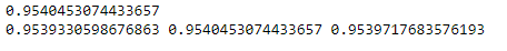
Now, we will be building a baseline model of svm which would take data with insignificant amount of data preprocessing which is to observe how our model is performing in non ideal situations.
le = LabelEncoder()
data['Activity'] = le.fit_transform(data.Activity)
X = data.iloc[:,:-1]
y = data.iloc[:,-1]
X_train, X_test, y_train, y_test = train_test_split(X, y, test_size=0.3, random_state=40)
classifier = SVC()
clf = classifier.fit(X_train, y_train)
y_pred = clf.predict(X_test)
precision, recall, f_score, _ = error_metric(y_test, y_pred, average = 'weighted')
model1_score = accuracy_score(y_test, y_pred)
print(model1_score)
print(precision, recall, f_score)
-
2.2 Feature selection and removing top correlated variables
We have near about 500+ features in our dataset. Not every feature contributes towards the model prediction hence we can cut down the no. of features according to their importance and then start a model building on top of it. This vague idea or process is called feature selection. We will be training a new scv model on new reduced dataset. We are reducing the features with the help of sklearn SelectFromModel. Lets see the accuracy metrics of this new trained model and shape of our new dataset.
lsvc = LinearSVC(C = 0.01, penalty="l1", dual=False, random_state=42).fit(X_train, y_train)
model_2 = SelectFromModel(lsvc, prefit=True)
new_train_features = model_2.transform(X_train)
new_test_features = model_2.transform(X_test)
print(new_train_features.shape,new_test_features.shape )
classifier_2 = SVC()
clf_2 = classifier_2.fit(new_train_features, y_train)
y_pred_new = clf_2.predict(new_test_features)
model2_score =accuracy_score(y_test, y_pred_new)
precision, recall, f_score, _ = error_metric(y_test, y_pred_new, average='weighted')
print(model2_score)
print(precision, recall, f_score)
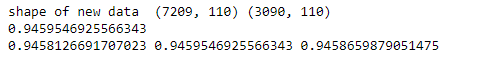
Observation
As we can see that our model is still working really well even after reduction of so many features. We have reduced features from 562 to 110 and you can compare the accuracy from previous model it is almost equivalent.
4. Hyperparameter Tuning for SVC with Grid Search and final model building.
Model hyperparmeters are configurations that is external to the model and whose value cannot be estimated from data. We will use gridsearch here with both rbf and linear kernel and value of C from 0.1 to 100.
parameters = {
    'kernel': ['linear', 'rbf'],
    'C': [100, 20, 1, 0.1]
}

selector = GridSearchCV(SVC(), parameters, scoring='accuracy')
selector.fit(new_train_features, y_train)

print('Best parameter set found:')
print(selector.best_params_)
print('Detailed grid scores:')
means = selector.cv_results_['mean_test_score']
stds = selector.cv_results_['std_test_score']
for mean, std, params in zip(means, stds, selector.cv_results_['params']):
    print('%0.3f (+/-%0.03f) for %r' % (mean, std * 2, params))
    print()

classifier_3 = SVC(kernel='rbf', C=100)
clf_3 = classifier_3.fit(new_train_features, y_train)
y_pred_final = clf_3.predict(new_test_features)
model3_score = accuracy_score(y_test, y_pred_final)

print('Accuracy score:', model3_score)
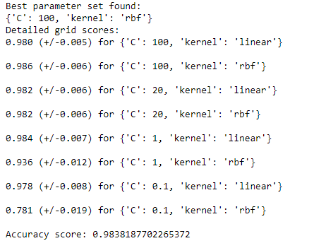
Observation:
As we can see this is the best hyperparameter {‘C’: 100, ‘kernel’: ‘rbf’} with accuracy of 98.38%
Code and Data
Full Code and Dataset can be found here
Conclusion and Future Work
Congratulations if you have reached her :) We can try tree based models such as random forest and GBDT. If You have any question regarding this blog feel free to contact me on my website