Problem

Twitter data is massive and as such analyzing twitter data is a mammoth undertaking. the cleaning and pre-processing of Twitter. Political polarization and reactions to new products are probably some of the biggest use-cases of twitter data analytics. We have dataset containing user tweets. These tweets can be negative (0) and positive (4). Based on the obtained data our goal is to identify the sentiment/polarity of the tweets.

About Dataset

There are 6 columns/features in the dataset and are described below:

• target: the polarity of the tweet (0 = negative, 4 = positive)
• ids: The id of the tweet ( ex :2087)
• date: the date of the tweet (ex: Sat May 16 23:58:44 UTC 2009)
• flag: The query (lyx). If there is no query, then this value is NO_QUERY.
• user: the user-name of the user that tweeted
• text: the text of the tweet

Importing libraries

import pandas as pd
import numpy as np
import os
import matplotlib.pyplot as plt
import seaborn as sns
from sklearn.model_selection import train_test_split
from sklearn.metrics import precision_recall_fscore_support as error_metric
from nltk.corpus import stopwords
import nltk
from string import punctuation
from nltk.stem.porter import *
from wordcloud import WordCloud
import matplotlib.pyplot as plt
from sklearn.feature_extraction.text import TfidfVectorizer
from sklearn.linear_model import LogisticRegression
from sklearn.model_selection import train_test_split
from sklearn.metrics import accuracy_score, classification_report
from vaderSentiment.vaderSentiment import SentimentIntensityAnalyzer
import warnings
warnings.filterwarnings('ignore')

EDA

• Loading Dataset ,checking for null values and sampling from data

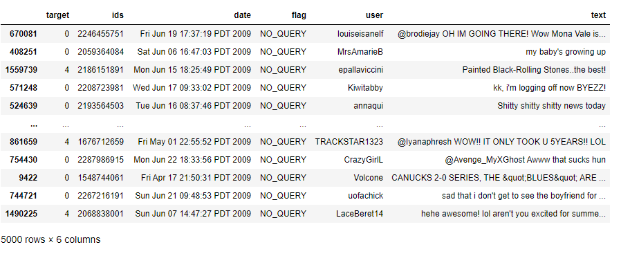
The first step - you know the drill by now - load the dataset and see how it looks like. In this task, we are basically looking for glimpse of overall data and look at the null values if they are present. Since the data 1600000 rows, We will be taking sample of 5000 tweets for the sake of easy computation power.

columns = ['target','ids','date','flag','user','text']
data = pd.read_csv('file.csv', encoding = 'latin-1', header = None)
data.columns = columns
data.shape
data = data.sample(n=5000, random_state=2)
data

Sentiment Analysis simplified

In layman’s terms sentiment analysis is basically figuring out the sentiment of a particular text. In the case with our problem statement, it is about finding out if a particular tweet is positive or negative, happy or unhappy (based on a score of course).

Approach towards dealing with sentiment analysis

The key to sentiment analysis is finding a number which indicates a level of positivity or negativity usually a number between 0 to 1, as it is obvious that computers cannot understand emotions such as happy or sad. However, a number could substitute an emotion and the value of this number signifies the magnitude of emotion in a direction; ex: very happy is above 0.9, happy is between 0.75 and 0.9, neutral is 0.5 and so on. The main challenge is how to obtain this number correctly with the help of given data.

In supervised setting you already have information as labels are already present in the training phase. First you would clean the data of unwanted substances like stopwords, punctuation marks etc. and then extract features by converting words into numbers. You can do this extraction step in various different ways like Bag-of-Words, TF-IDF with or without n-grams approach. Then you feed some sort of classifier which outputs a labels based on some internal scoring mechanism.

Why use sentiment analysis?

It’s estimated that 80% of the world’s data is unstructured and not organized in a pre-defined manner. Most of this comes from text data, like emails, support tickets, chats, social media, surveys, articles, and documents. These texts are usually difficult, time-consuming and expensive to analyze, understand, and sort through.

Sentiment analysis systems allows companies to make sense of this sea of unstructured text by automating business processes, getting actionable insights, and saving hours of manual data processing, in other words, by making teams more efficient.

With the help of sentiment analysis, unstructured information could be automatically transformed into structured data of public opinions about products, services, brands, politics, or any topic that people can express opinions about. This data can be very useful for commercial applications like marketing analysis, public relations, product reviews, net promoter scoring, product feedback, and customer service.

Issues with sentiment analysis

Computers have a hard time carrying out sentiment analysis tasks. Some pressing issues with performing sentiment analysis are:

• Sarcasm: It is one of the most difficult sentiments to interpret properly. Example: “It was awesome for the week that it worked.”
• Relative sentiment: It is not a classic negative, but can be a negative nonetheless. Example: “I bought an iPhone” is good for Apple, but not for other mobile companies.
• Compound or multidimensional sentiment: These types contain positives and negatives in the same phrase. Example: “I love Mad Men, but hate the misleading episode trailers.” The above sentence consists of two polarities, i.e., Positive as well as Negative. So how do we conclude whether the review was Positive or Negative?
• Use of emoticons: Heavy use of emoticons (which have sentiment values) in social media texts like that of Twitter and Facebook also makes text analysis difficult.

Data Preprocessing

• Tackling user handles

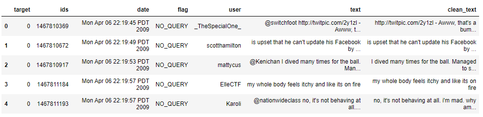
Tweets can be directed to any other person with username/user handle “NAME” @NAME. Consider the tweet ‘@brodiejay OH IM GOING THERE! Wow Mona Vale is a real place afterall! I know it sucks Mville only does the slow train pffft ‘. Here, ‘@brodiejay’ is the user handle or username of the person to whom that particular tweet was directed/referred. If you take another tweet “my baby’s growing up “, it doesn’t contain any such user handle. So, in the dataset, user handles are present, but not in all observations.

From basic intuition it is clear that user handles have little to zero contribution towards sentiment formation. So, it is a good idea to remove them altogether from the data. Getting rid of user handles also helps in reduction of the term-frequency matrix that gets generated. This will directly boost up calculation speed and also performance as unnecessary features will not be generated. Below code will clean our tweets.

def remove_pattern(input_txt, pattern):
    r = re.findall(pattern, input_txt)
    for i in r:
        input_txt = re.sub(i, '', input_txt)

    return input_txt  
data['clean_text'] = data['text'].apply(lambda row:remove_pattern(row, "@[\w]*"))

data.head(5)

• Text Preprocessing

This data can now be further preprocessed of unwanted entries which will make the data more suitable for carrying out analysis. Below discussed in brief are the preprocessing techniques that you will be carrying out at the end of this topic.

• Tokenization- Tokenization describes splitting paragraphs into sentences, or sentences into individual pieces called tokens. Words, numbers, punctuation marks, and others can be considered as tokens. Most of what we are going to do with language relies on first separating out such tokens separately so that subsequent preprocessing steps can be successfully done.

• Stopwords removal- Stopwords are the most common words in a language like ‘the’, ‘a’, ‘on’, ‘is’, ‘all’. These words do not carry important meaning and so are usually removed from texts.

• Stemming- Much of natural language machine learning is about sentiment of the text. Stemming is a process of reducing words to their word stem, base or root form (for example, books — book, looked — look). The main two algorithms are Porter stemming algorithm (removes common morphological and inflexional endings from words and Lancaster stemming algorithm (a more aggressive stemming algorithm). Below Code will tokenize our clean text then removing stopwords from nltk, after that we will aply stemming.

stop_words = list(set(stopwords.words('english')))+list(punctuation)+['``', "'s", "...", "n't"]
data['tokenized_text'] = [nltk.word_tokenize(x) for x in data['clean_text']]
data['tokenized_text'] = data['tokenized_text'].apply(lambda row: [word for word in row if word not in stop_words])
stemmer = PorterStemmer()
data['tokenized_text'] = data['tokenized_text'].apply(lambda x: [stemmer.stem(i) for i in x])
data['tokenized_text'] = data['tokenized_text'].apply(lambda x: ' '.join(x))
data.head()

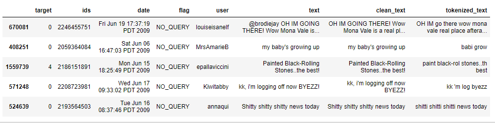
Observation:

As you can see tokenized_text’s 1st row is converted into “OH IM go there” from “OH IM GOING THERE!”

Word Cloud

• Word cloud of all data

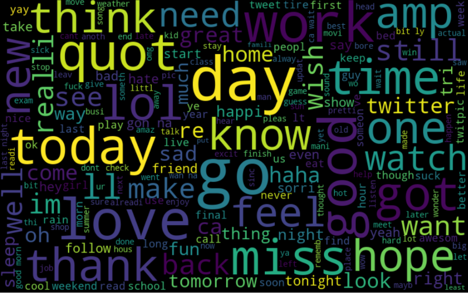
It is a visualisation method that displays how frequently words appear in a given body of text, by making the size of each word proportional to its frequency. All the words are then arranged in a cluster or cloud of words. Alternatively, the words can also be arranged in any format: horizontal lines, columns or within a shape.

Now that you have an idea about how to use a wordcloud, lets do a simple task to generate a wordcloud to observe the most frequently occuring words.

all_words = ' '.join([text for text in data['tokenized_text']])
# generate wordcloud object
wordcloud = WordCloud(width=800, height=500, random_state=21, max_font_size=110).generate(all_words)
plt.figure(figsize=(20, 12))
plt.imshow(wordcloud, interpolation="bilinear")
plt.axis('off')
plt.show()

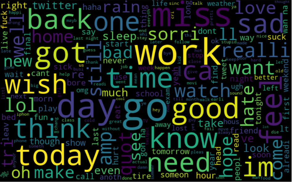
• Word cloud for negative data

# negative tweets
neg_words = ' '.join([text for text in data['tokenized_text'][data['target'] == 0]])

# generate wordcloud object for negative tweets
neg_wordcloud = WordCloud(width=800, height=500, random_state=21, max_font_size=110).generate(neg_words)
plt.figure(figsize=(20, 12))
plt.imshow(neg_wordcloud, interpolation="bilinear")
plt.axis('off')
plt.show()

• Word cloud for postive data

# positive tweets
pos_words = ' '.join([text for text in data['tokenized_text'][data['target'] == 4]])

# generate wordcloud object for negative tweets
pos_wordcloud = WordCloud(width=800, height=500, random_state=21, max_font_size=110).generate(pos_words)
plt.figure(figsize=(20, 12))
plt.imshow(pos_wordcloud, interpolation="bilinear")
plt.axis('off')
plt.show()

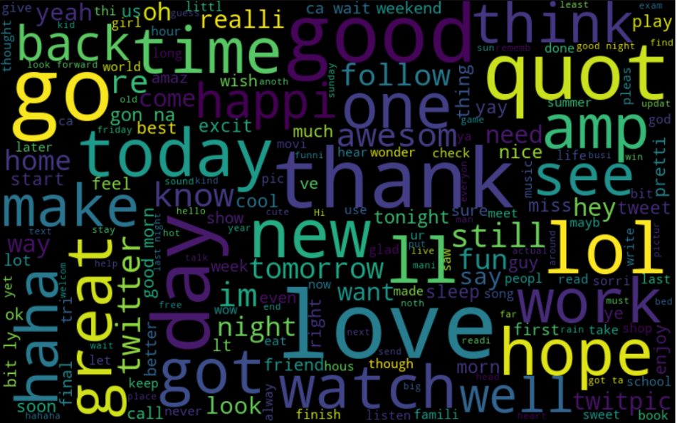
Observation:

As you can see in negative word cloud there are lots of negative words such as fuck, bad, tire etc and in postive word cloud there are many good words.

Model Building

Logistic Regression for predicting sentiments These steps enabled us with data in proper format as well as some interesting insights about certain keywords. This cleaned form of data can now be fed to a machine learning algorithm to classify tweets into categories. Since we are already familiar with the workflow of classifying texts, we will be only outlining the steps associated with it. The steps are as follows:

• Splitting into training and test sets
• Construct a term-document matrix (can be done by Bag of Words or TF-IDF)
• Fitting a classifier on training data
• Predicting on test data
• Evaluating classifier performance

# ratio to split into training and test set
ratio = int(len(data)*0.75)

# logistic regression model
logreg = LogisticRegression(random_state=2)

# TF-IDF feature matrix
tfidf_vectorizer = TfidfVectorizer(max_df=0.90, min_df=2, max_features=1000, stop_words='english')

# fit and transform tweets
tweets = tfidf_vectorizer.fit_transform(data['tokenized_text'])

# convert positive tweets to 1's
data['target'] = data['target'].apply(lambda x: 1 if x==4 else x)

# split into train and test
X_train = tweets[:ratio,:]
X_test = tweets[ratio:,:]
y_train = data['target'].iloc[:ratio]
y_test = data['target'].iloc[ratio:]

# fit on training data
logreg.fit(X_train,y_train)

# make predictions
prediction = logreg.predict_proba(X_test)
prediction_int = prediction[:,1] >= 0.3
prediction_int = prediction_int.astype(np.int)
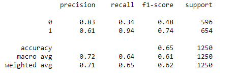
report = classification_report(y_test,prediction_int)

# print out classification_report
print(report)

TextBlob

There are numerous libraries out there for dealing with text data. One of them is TextBlob which is built on the shoulders of NLTK and Pattern. A big advantage of TextBlob is it is easy to learn and offers a lot of features like sentiment analysis, pos-tagging, noun phrase extraction, etc. It has now become a go-to library for many users who are performing NLP tasks.

Features of TextBlob

The documentation page of TextBlob says; TextBlob aims to provide access to common text-processing operations through a familiar interface. You can treat TextBlob objects as if they were Python strings that learned how to do Natural Language Processing.

• Sentiment Analysis with TextBlob

You can carry out sentiment analysis with textBlob too. The TextBlob object has an attribute sentiment that returns a tuple of the form Sentiment (polarity, subjectivity). The polarity score is a float within the range [-1.0, 1.0] with negative values corresponding to negative sentiments and positive values to positive sentiments. The subjectivity is a float within the range [0.0, 1.0] where 0.0 is very objective and 1.0 is very subjective.

But how it does this prediction of sentiment scoring? Well, it has a training set with preclassified movie reviews, so when you give a new text for analysis, it uses NaiveBayes classifier to classify the new text’s polarity in pos and neg probabilities.

# list to store polarities
tb_polarity = []

# loop over tweets
for sentence in data['tokenized_text']:
    temp = TextBlob(sentence)
    tb_polarity.append(temp.sentiment[0])

# new column to store polarity    
data['tb_polarity'] = tb_polarity
data.head(10)

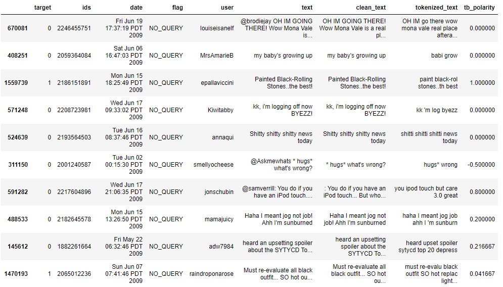
Observation

You can compare the target values with tb_polarity and see how much TextBlob is accurate

VaderSentiment

Another library for out of the box sentiment analysis is vaderSentiment. It is an open sourced python library where VADER stands for Valence Aware Dictionary and sEntiment Reasoner. With VADER you can be up and running performing sentiment classification very quickly even if you don’t have positive and negative text examples to train a classifier or want to write custom code to search for words in a sentiment lexicon. VADER is also computationally efficient when compared to other Machine Learning and Deep Learning approaches.

VADER performs well on text originating in social media and is described fully in a paper entitled VADER: A Parsimonious Rule-based Model for Sentiment Analysis of Social Media Text. published at ICWSM-14. VADER is able to include sentiment from emoticons (e.g, :-)), sentiment-related acronyms (e.g, LOL) and slang (e.g, meh). The developers of VADER have used Amazon’s Mechanical Turk to get most of their ratings, You can find complete details on their Github Page.

Output of VADER

VADER produces four sentiment metrics from these word ratings. The first three metrics; positive, neutral and negative, represent the proportion of the text that falls into those categories. The final metric, the compound score, is the sum of all of the lexicon ratings which have been standardised to range between -1 and 1.

How does VADER work?

First step is to import SentimentIntensityAnalyzer from vaderSentiment.vaderSentiment. Then initialize an object of SentimentIntensityAnalyzer() and use its .polarity_scores() on a given text to find about its four metrics. Below given is a code snippet:

analyser = SentimentIntensityAnalyzer()

# empty list to store VADER polarities
vs_polarity = []

# loop over tweets
for sentence in data['tokenized_text']:
    vs_polarity.append(analyser.polarity_scores(sentence)['compound'])

# add new column `'vs_polarity'` to data
data['vs_polarity'] = vs_polarity

data.head(10)

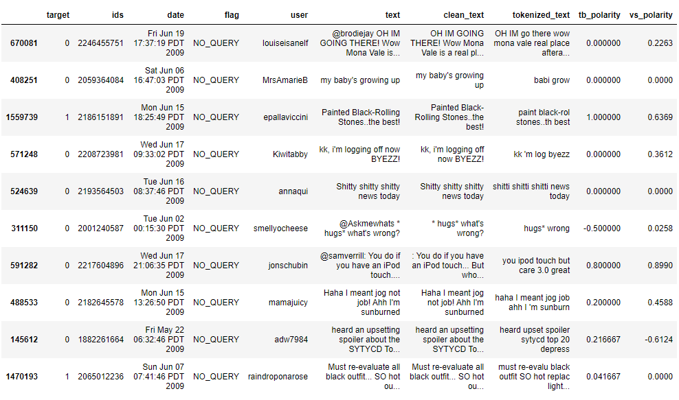
Observation:

you can also compare the vs_polarity to the target variables.

Code and Data

Full Code and Dataset can be found here

Conclusion and Future Work

Congratulations if you have reached her :) We can try tree based models such as random forest and GBDT and other types of feature transformation such as word2vec. If You have any question regarding this blog feel free to contact me on my website

Reference

• https://greyatom.com/