Problem Statement
Credit scoring algorithms, which makes a guess at the probability of default, are the method banks use to determine whether or not a loan should be granted. We will predicting the probability that somebody will experience financial distress in the next two years.
Dataset
| Feature | Description |
|---|---|
| SeriousDlqin2yrs | Person experienced 90 days past due delinquency or worse |
| RevolvingUtilizationOfUnsecuredLines | Total balance on credit cards and personal lines of credit |
| age | Age of borrower in years |
| NumberOfTime30-59DaysPastDueNotWorse | Number of times borrower has been 30-59 days past due but no worse in the last 2 years |
| DebtRatio | Monthly debt payments, alimony,living costs divided by monthy gross income |
| MonthlyIncome | Monthly Income |
| NumberOfOpenCreditLinesAndLoans | Number of Open loans (installment like car loan or mortgage) and Lines of credit |
| NumberOfTimes90DaysLate | Number of times borrower has been 90 days or more past due |
| NumberRealEstateLoansOrLines | Number of mortgage and real estate loans including home equity lines of credit |
| NumberOfTime60-89DaysPastDueNotWorse | Number of times borrower has been 60-89 days past due but no worse in the last 2 years |
| NumberOfDependents | Number of dependents in family excluding themselves |
Importing libraries
import pandas as pd
import numpy as np
import os
import matplotlib.pyplot as plt
import seaborn as sns
from sklearn.model_selection import train_test_split
from sklearn.preprocessing import StandardScaler
from sklearn.metrics import accuracy_score
from sklearn.linear_model import LogisticRegression
from sklearn.metrics import roc_auc_score
from sklearn import metrics
import matplotlib.pyplot as plt
from sklearn.metrics import f1_score, confusion_matrix, classification_report
from sklearn.metrics import precision_score, recall_score
from imblearn.over_sampling import SMOTE
from sklearn.ensemble import RandomForestClassifier
import warnings
warnings.filterwarnings('ignore')
1. EDA
-
1.1 Loading Dataset and splitting into train test sets
First we’ll load the dataset with pandas and split it into X and y variable where X contains our features and y contains our target variable. This can be done by the following code
df = pd.read_csv('financial.csv').drop('Unnamed: 0',1)
X = df.drop(['SeriousDlqin2yrs'],axis = 1)
y = df['SeriousDlqin2yrs']
count = y.value_counts()
X_train,X_test,y_train,y_test = train_test_split(X,y,test_size = 0.3,random_state = 6)
-
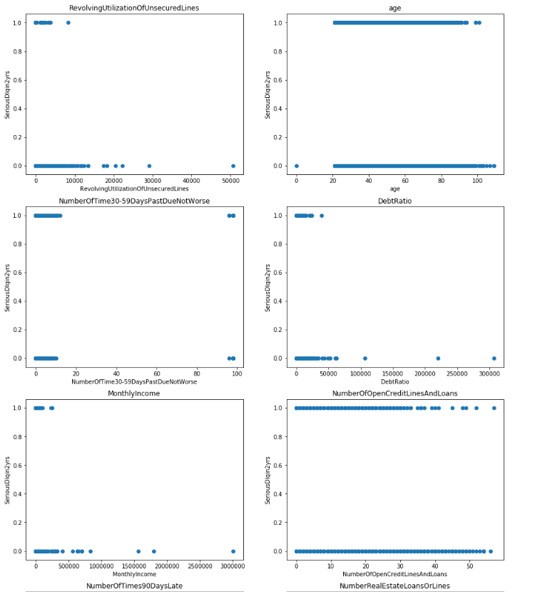
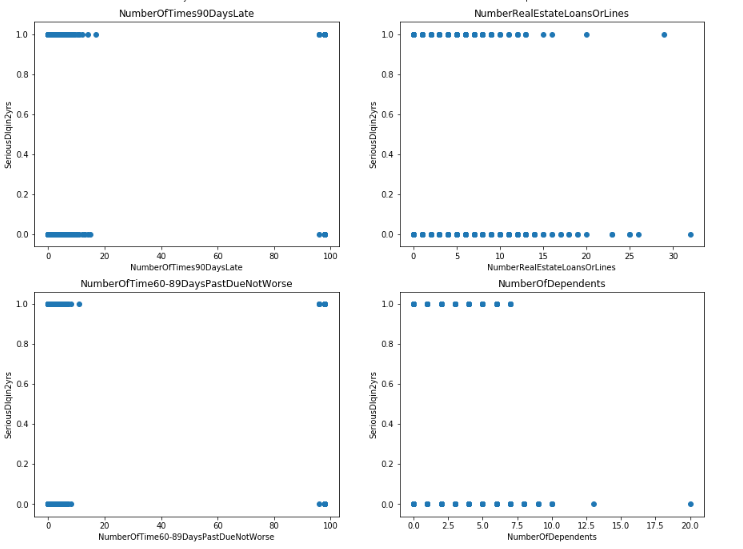
1.2 Visualising the data
Visualization is an important part as you can get an idea of the data just by looking at different graphs. We will try to get an idea of how our features are related to the dependent variable and get some insights about the data using scatter plot. The below code will do that.
cols = list(X.columns)
fig, axes = plt.subplots(nrows=5, ncols=2, figsize=(10,25))
for i in range(0,5):
    for j in range(0,2):
        col= cols[i * 2 + j]
        axes[i,j].set_title(col)
        axes[i,j].scatter(X_train[col],y_train)
        axes[i,j].set_xlabel(col)
        axes[i,j].set_ylabel('SeriousDlqin2yrs')
-
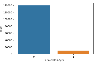
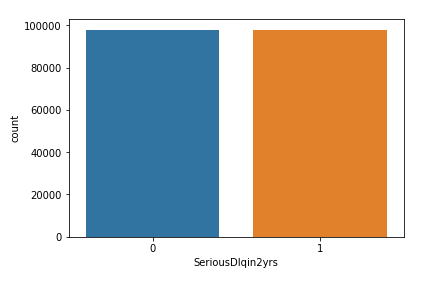
1.3 Value count of classes
As we can see our dataset is highly imbalanced
sns.countplot(df['SeriousDlqin2yrs'])
2. Data Preprocessing
-
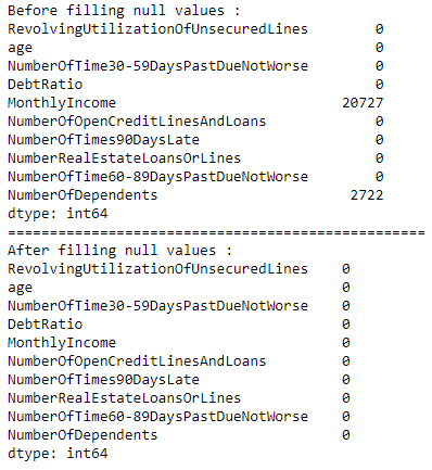
2.1 Checking for missing values and replace it with appropriate values
Real-world data often has missing values. Data can have missing values for a number of reasons such as observations that were not recorded and data corruption. Handling missing data is important as many machine learning algorithms do not support data with missing values. We will check for missing values and replace them with appropriate values.The below code will do the task.
print(X_train.isnull().sum())
X_train['MonthlyIncome'].fillna(X_train['MonthlyIncome'].median(),inplace = True)
X_train['NumberOfDependents'].fillna(X_train['NumberOfDependents'].median(),inplace = True)
X_test['MonthlyIncome'].fillna(X_test['MonthlyIncome'].median(),inplace = True)
X_test['NumberOfDependents'].fillna(X_test['NumberOfDependents'].median(),inplace = True)
print(X_test.isnull().sum())
-
2.2 Feature selection
We always try to reduce our features to the minimum number of most significant features. The basic rule of feature selection is that we need to select features which are highly correlated to the dependent variable and also not highly correlated with each other as they show the same trend. We do this with the help of the correlation matrix. So, we will find the features which are highly correlated and select the most significant features amongst them.
corr = X_train.corr()
plt.figure(figsize=(14,12))
sns.heatmap(corr, annot=True, fmt=".2g")
X_train.drop(['NumberOfTime30-59DaysPastDueNotWorse','NumberOfTime60-89DaysPastDueNotWorse'],axis = 1,inplace=True)
X_test.drop(['NumberOfTime30-59DaysPastDueNotWorse','NumberOfTime60-89DaysPastDueNotWorse'],axis = 1,inplace=True)

print(X_train.columns)
print(X_test.columns)
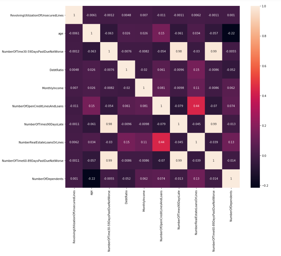
Observation:
As we can see from the heat map that the features NumberOfTime30-59DaysPastDueNotWorse, NumberOfTimes90DaysLate and NumberOfTime60-89DaysPastDueNotWorse are highly correlated. So we are dropping NumberOfTime30-59DaysPastDueNotWorse and NumberOfTime60-89DaysPastDueNotWorse from X_train and X_test as well.
-
2.3 Scaling the features
While working with the learning model, it is important to scale the features to a range which is centered around zero so that the variance of the features are in the same range. If the feature’s variance is orders of magnitude more than the variance of other features, that particular feature might dominate other features in the dataset and our model will not train well which gives us bad model.
scaler = StandardScaler()
X_train = scaler.fit_transform(X_train)
X_test = scaler.transform(X_test)
3. Model
-
3.1 Predict the values after building a Machine learning model
Logistic regression is another technique borrowed by machine learning from the field of statistics.It is the go-to method for binary classification problems (problems with two class values). In this post we will discover the logistic regression algorithm for machine learning.This is a classification problem to predict whether somebody will face financial distress in the next two years. So, here we will train our data on a Logistic regression algorithm and try to correctly predict the class.
log_reg = LogisticRegression()
log_reg.fit(X_train,y_train)
y_pred = log_reg.predict(X_test)
accuracy = accuracy_score(y_test,y_pred)
-
3.2 Is our prediction right?
Simply, building a predictive model is not your motive. But, creating and selecting a model which gives high accuracy. Hence, it is crucial to check accuracy of the model and we consider different kinds of metrics to evaluate our models. The choice of metric completely depends on the type of model and the implementation plan of the model. After you are finished building your model, these metrics will help you in evaluating your model accuracy.We will print the classification report of our model. This can be done by the following code
score = roc_auc_score(y_pred , y_test)
y_pred_proba = log_reg.predict_proba(X_test)[:,1]
fpr, tpr, _ = metrics.roc_curve(y_test,  y_pred_proba)
auc = metrics.roc_auc_score(y_test, y_pred_proba)
plt.plot(fpr,tpr,label="Logistic model, auc="+str(auc))
plt.xlabel('False Positive Rate')
plt.ylabel('True Positive Rate')
plt.legend(loc=4)
plt.show()
f1 = f1_score(y_test, log_reg.predict(X_test))
precision = precision_score(y_test, log_reg.predict(X_test))
recall = recall_score(y_test, log_reg.predict(X_test))
roc_auc = roc_auc_score(y_test, log_reg.predict(X_test))
print ('Confusion_matrix' + '\n', confusion_matrix(y_test, log_reg.predict(X_test)))
print ('Classification_report' + '\n' + classification_report(y_test,y_pred))
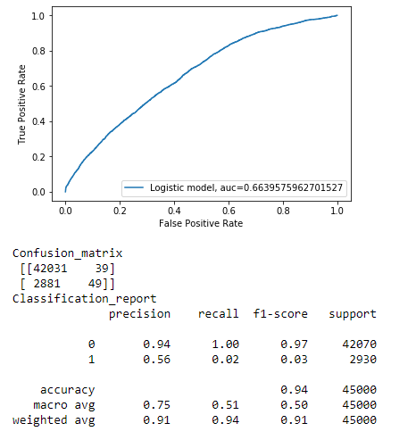
Observation:
As we can see our model is not working well in calss 1 category because this is an imbalanced data we will now try to fix this. Auc metric helps us to determine if our model is working well in imabalnced class.
4. SMOTE
-
4.1 Balancing the dataset using SMOTE
As we can see that the dataset is not balanced and it shows that 93% of customers will not face financial distress.In this situation, the predictive model developed using conventional machine learning algorithms could be biased and inaccurate.This happens because Machine Learning Algorithms are usually designed to improve accuracy by reducing the error. Thus, they do not take into account the class distribution / proportion or balance of classes. If we train our model on such an imbalanced data we will get incorrect predictions. To overcome this there are different methods such undersampling, oversampling and SMOTE. We will be using the SMOTE technique.Check for different evaluation metrics.
count = y.value_counts()
smote = SMOTE(random_state=9)
X_sample, y_sample = smote.fit_sample(X_train, y_train)
sns.countplot(y_sample)
Observation:
As we can see now our dataset is balanced now. Lets try applying new model on this dataset.
-
4.2 Effect of applying SMOTE?
SMOTE is an over-sampling method. What it does is, it creates synthetic (not duplicate) samples of the minority class. Hence making the minority class equal to the majority class. After applying ‘SMOTE’ we have balanced the data. We will use this balanced data for training our model and check whether the performance of our model has improved or not by comparing different evaluation parameters.
log_reg.fit(X_sample, y_sample)
y_pred = log_reg.predict(X_test)
score = roc_auc_score(y_pred , y_test)
y_pred_proba = log_reg.predict_proba(X_test)[:,1]
fpr, tpr, _ = metrics.roc_curve(y_test,  y_pred_proba)
auc = metrics.roc_auc_score(y_test, y_pred_proba)
plt.plot(fpr,tpr,label="Logistic model, auc="+str(auc))
plt.xlabel('False Positive Rate')
plt.ylabel('True Positive Rate')
plt.legend(loc=4)
plt.show()
f1 = f1_score(y_test, log_reg.predict(X_test))
precision = precision_score(y_test, log_reg.predict(X_test))
recall = recall_score(y_test, log_reg.predict(X_test))
# roc_auc = roc_auc_score(y_test, log_reg.predict(X_test))
print('Confusion matrix' + '\n' ,confusion_matrix(y_test, log_reg.predict(X_test)))
print ('Classification_report' + '\n' + classification_report(y_test,y_pred))
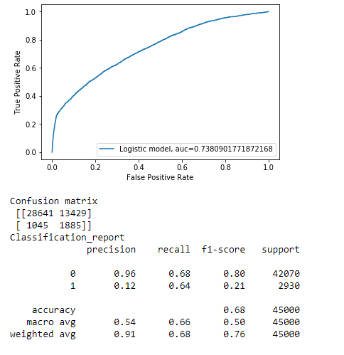
Observation:
If you compare previos classification report to this one you can observe that our model has imporved pretty much for our minority class. F1 score of class 1 has been improved from 3% to 21% , thats quite an improvemnt!! See the power of SMOTE.
5. Random Forest Algorithm
Random Forrest is a bagging technique which uses Decision Tree as the base model. The performance of our Logistic regression model has signifiacntly improved after balancing the data, lets check can we furthur improve it by using a Random Forrest model.
rf = RandomForestClassifier(random_state=9)
rf.fit(X_sample, y_sample)
y_pred = rf.predict(X_test)
f1 = f1_score(y_test, rf.predict(X_test))
precison = precision_score(y_test, rf.predict(X_test))
recall = recall_score(y_test, rf.predict(X_test))
score = roc_auc_score(y_test, rf.predict(X_test))
print ('Confusion_matrix' + '\n',confusion_matrix(y_test, rf.predict(X_test)))
print ('Classification_report' + '\n' + classification_report(y_test,y_pred))
score = roc_auc_score(y_pred , y_test)
y_pred_proba = rf.predict_proba(X_test)[:,1]
fpr, tpr, _ = metrics.roc_curve(y_test,  y_pred_proba)
auc = metrics.roc_auc_score(y_test, y_pred_proba)
plt.plot(fpr,tpr,label="Random_forest model, auc="+str(auc))
plt.xlabel('False Positive Rate')
plt.ylabel('True Positive Rate')
plt.legend(loc=4)
plt.show()
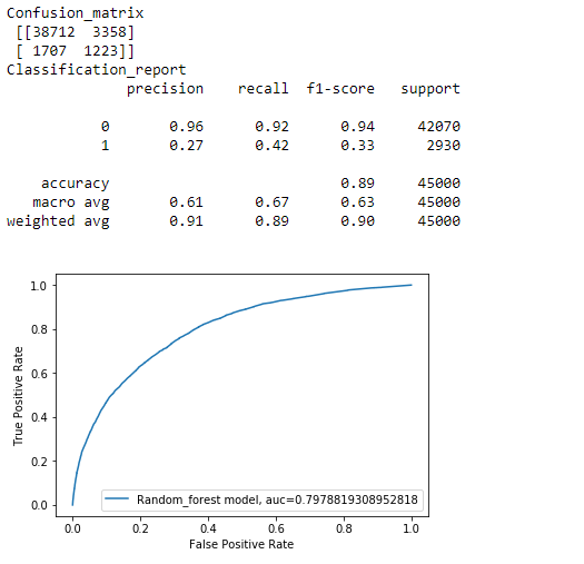
Observation:
As you can see our model has been improved.F1 score of class 1 increased from 21% to 33%.
Code and Data
Full Code and Dataset can be found here
Conclusion and Future Work
Congratulations if you have reached her :) You can try to increase the f1 score of minority class by hyperparameter tuning of random forest. Also you can try using xgboost. If You have any question regarding this blog feel free to contact me on my website